Decision Boundaries in KNN
What is a Decision Boundary?
The boundary where the model changes its prediction from one class to another.For example:
Left Side  → Class Red

Right Side → Class Blue
The separating line is called the decision boundary.
Decision Boundary in Linear Models
Consider a Linear SVM or Logistic Regression model.
Red Class       |      Blue Class
Red Class       |      Blue Class
Red Class       |      Blue Class
The boundary is:
Straight Line
Linear models always create:
Linear Decision Boundary
Decision Boundary in KNN
KNN does not create a fixed mathematical equation.
Instead:
New Point
      ↓
Find Nearest Neighbors
      ↓
Majority Voting
      ↓
Predict Class
Because every prediction depends on nearby points, the boundary can become:
Curved
Irregular
Complex
Therefore:
KNN creates Non-Linear Decision Boundaries
Example Dataset
Consider the following data:
Red Points

(1,1)
(2,1)
(1,2)

Blue Points

(5,5)
(6,5)
(5,6)
Visual representation:
y

6 |                  B
5 |               B     B
4 |
3 |
2 | R
1 | R     R
0 +-------------------------
    0 1 2 3 4 5 6      x
Where:
R = Red
B = Blue
How KNN Creates Decision Regions
Imagine placing a new point anywhere on the graph.
KNN asks:
Who are my nearest neighbors?
If most nearest neighbors are:
Red
Prediction:
Red
If most nearest neighbors are:
Blue
Prediction:
Blue
As we repeat this for every possible location:
Feature Space
gets divided into regions.
These regions form the:
Decision Boundary
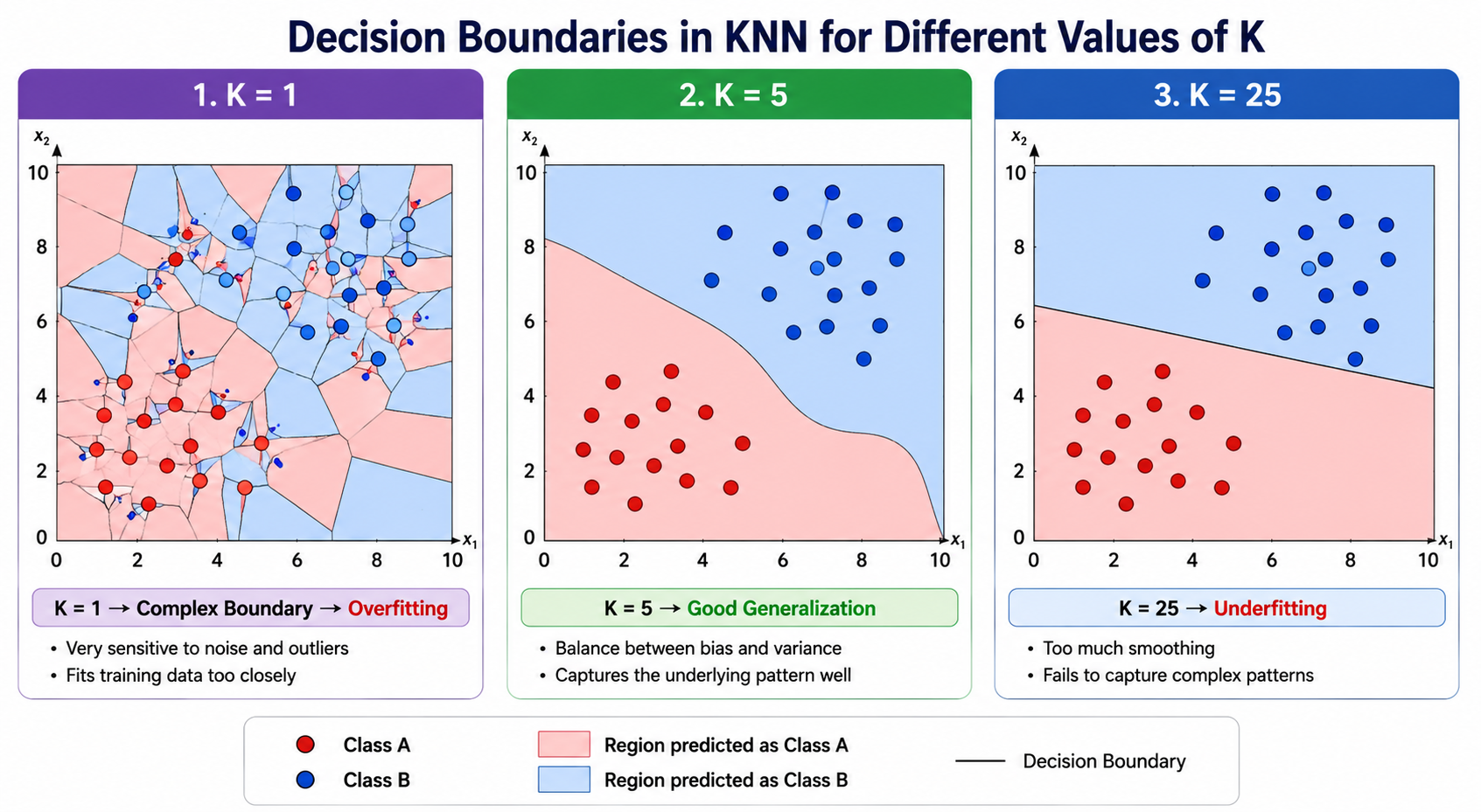
Effect of K on Decision Boundary
Small K
Example:
K = 1
Characteristics:
Complex Boundary
Sensitive to Noise
High Variance
Overfitting
Medium K
Example:
K = 5
Characteristics:
Balanced Boundary
Good Generalization
Large K
Example:
K = 25
Characteristics:
Very Smooth Boundary
High Bias
Underfitting
Visual Comparison
K = 1
Many Zig-Zag Regions

\/\/\/\/\/\/\/\/
Decision boundary is very irregular.
K = 5
Gentle Curves

~~~~~~~~~~~~~
Decision boundary becomes smoother.
K = 25
Almost Straight

--------------
Boundary becomes overly simplified.
Why KNN Can Solve Non-Linear Problems
Suppose the classes form a circle.
Inside Circle  → Red

Outside Circle → Blue
A straight line cannot separate them.
Linear models fail.
But KNN checks local neighborhoods.
So KNN naturally creates:
Circular Boundary
and classifies correctly.
This is the biggest advantage of KNN.
Real-Life Analogy
Imagine moving into a new neighborhood.
You want to know whether the area is:
Residential
or
Commercial
You ask nearby buildings.
If most nearby buildings are residential:
Prediction = Residential
If most nearby buildings are commercial:
Prediction = Commercial
The neighborhood boundaries emerge naturally from local information.
This is exactly how KNN creates decision boundaries.
Decision Boundary and Bias-Variance Tradeoff
| K Value | Boundary Type | Bias | Variance |
|---|---|---|---|
| Small K | Complex | Low | High |
| Medium K | Balanced | Balanced | Balanced |
| Large K | Smooth | High | Low |
This is one reason K selection is very important in KNN.
Important Points
- A decision boundary separates different classes.
- KNN creates decision boundaries using neighboring points.
- KNN does not learn a fixed equation.
- Small K creates complex boundaries.
- Large K creates smooth boundaries.
- KNN can generate non-linear decision boundaries.
- KNN can solve problems where linear classifiers fail.
- K value controls boundary complexity.
- Decision boundaries explain why KNN is a non-linear classifier.
Keywords
KNN Decision Boundary, Non Linear Classification, K Nearest Neighbors, Decision Regions, K Value Effect, Overfitting in KNN, Underfitting in KNN, Bias Variance Tradeoff, Local Classification, Machine Learning Decision Boundary