
Example: MLR
Multiple Linear Regression — Complete Mathematical Example
Problem Statement
We want to predict y using two input variables:
X1 and X2
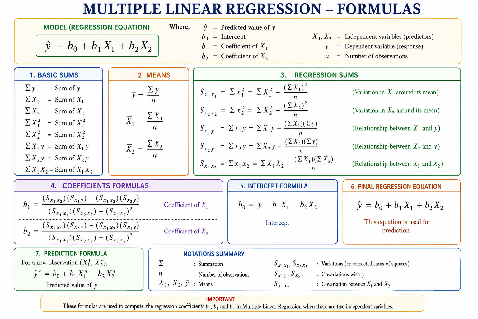
The Multiple Linear Regression equation is:
ŷ = b0 + b1X1 + b2X2
Where:
ŷ  = Predicted value
b0 = Intercept
b1 = Coefficient of X1
b2 = Coefficient of X2
Dataset
| y | X1 | X2 |
|---|---|---|
| 140 | 60 | 22 |
| 155 | 62 | 25 |
| 159 | 67 | 24 |
| 179 | 70 | 20 |
| 192 | 71 | 15 |
| 200 | 72 | 14 |
| 212 | 75 | 14 |
| 215 | 78 | 11 |
Step 1: Create Additional Columns
We need to calculate:
X1², X2², X1Y, X2Y, X1X2
| y | X1 | X2 | X1² | X2² | X1Y | X2Y | X1X2 |
|---|---|---|---|---|---|---|---|
| 140 | 60 | 22 | 3600 | 484 | 8400 | 3080 | 1320 |
| 155 | 62 | 25 | 3844 | 625 | 9610 | 3875 | 1550 |
| 159 | 67 | 24 | 4489 | 576 | 10653 | 3816 | 1608 |
| 179 | 70 | 20 | 4900 | 400 | 12530 | 3580 | 1400 |
| 192 | 71 | 15 | 5041 | 225 | 13632 | 2880 | 1065 |
| 200 | 72 | 14 | 5184 | 196 | 14400 | 2800 | 1008 |
| 212 | 75 | 14 | 5625 | 196 | 15900 | 2968 | 1050 |
| 215 | 78 | 11 | 6084 | 121 | 16770 | 2365 | 858 |
Step 2: Calculate Column Sums
n = 8
Σy = 140 + 155 + 159 + 179 + 192 + 200 + 212 + 215
Σy = 1452
ΣX1 = 60 + 62 + 67 + 70 + 71 + 72 + 75 + 78
ΣX1 = 555
ΣX2 = 22 + 25 + 24 + 20 + 15 + 14 + 14 + 11
ΣX2 = 145
ΣX1² = 3600 + 3844 + 4489 + 4900 + 5041 + 5184 + 5625 + 6084
ΣX1² = 38767
ΣX2² = 484 + 625 + 576 + 400 + 225 + 196 + 196 + 121
ΣX2² = 2823
ΣX1Y = 8400 + 9610 + 10653 + 12530 + 13632 + 14400 + 15900 + 16770
ΣX1Y = 101895
ΣX2Y = 3080 + 3875 + 3816 + 3580 + 2880 + 2800 + 2968 + 2365
ΣX2Y = 25364
ΣX1X2 = 1320 + 1550 + 1608 + 1400 + 1065 + 1008 + 1050 + 858
ΣX1X2 = 9859
Step 3: Calculate Means
mean_y = Σy / n
mean_y = 1452 / 8
mean_y = 181.5
mean_X1 = ΣX1 / n
mean_X1 = 555 / 8
mean_X1 = 69.375
mean_X2 = ΣX2 / n
mean_X2 = 145 / 8
mean_X2 = 18.125
Step 4: Calculate Regression Sums
Regression sums help measure the variation and relationship between variables after removing the effect of means.
We need:
Σx1², Σx2², Σx1y, Σx2y, Σx1x2
Calculate Σx1²
Formula:
Σx1² = ΣX1² - ((ΣX1)² / n)
Substitute values:
Σx1² = 38767 - ((555)² / 8)
Σx1² = 38767 - (308025 / 8)
Σx1² = 38767 - 38503.125
Σx1² = 263.875
Calculate Σx2²
Formula:
Σx2² = ΣX2² - ((ΣX2)² / n)
Substitute values:
Σx2² = 2823 - ((145)² / 8)
Σx2² = 2823 - (21025 / 8)
Σx2² = 2823 - 2628.125
Σx2² = 194.875
Calculate Σx1y
Formula:
Σx1y = ΣX1Y - ((ΣX1)(Σy) / n)
Substitute values:
Σx1y = 101895 - ((555)(1452) / 8)
Σx1y = 101895 - (805860 / 8)
Σx1y = 101895 - 100732.5
Σx1y = 1162.5
Calculate Σx2y
Formula:
Σx2y = ΣX2Y - ((ΣX2)(Σy) / n)
Substitute values:
Σx2y = 25364 - ((145)(1452) / 8)
Σx2y = 25364 - (210540 / 8)
Σx2y = 25364 - 26317.5
Σx2y = -953.5
Calculate Σx1x2
Formula:
Σx1x2 = ΣX1X2 - ((ΣX1)(ΣX2) / n)
Substitute values:
Σx1x2 = 9859 - ((555)(145) / 8)
Σx1x2 = 9859 - (80475 / 8)
Σx1x2 = 9859 - 10059.375
Σx1x2 = -200.375
Step 5: Calculate b1
Formula:
b1 = (((Σx2²)(Σx1y)) - ((Σx1x2)(Σx2y))) / (((Σx1²)(Σx2²)) - ((Σx1x2)²))
Substitute values:
b1 = (((194.875)(1162.5)) - ((-200.375)(-953.5))) / (((263.875)(194.875)) - ((-200.375)²))
Calculate numerator:
(194.875)(1162.5) = 226545.9375
(-200.375)(-953.5) = 191063.5625
Numerator = 226545.9375 - 191063.5625
Numerator = 35482.375
Calculate denominator:
(263.875)(194.875) = 51422.640625
(-200.375)² = 40150.140625
Denominator = 51422.640625 - 40150.140625
Denominator = 11272.5
Now calculate b1:
b1 = 35482.375 / 11272.5
b1 = 3.148
Step 6: Calculate b2
Formula:
b2 = (((Σx1²)(Σx2y)) - ((Σx1x2)(Σx1y))) / (((Σx1²)(Σx2²)) - ((Σx1x2)²))
Substitute values:
b2 = (((263.875)(-953.5)) - ((-200.375)(1162.5))) / (((263.875)(194.875)) - ((-200.375)²))
Calculate numerator:
(263.875)(-953.5) = -251605.8125
(-200.375)(1162.5) = -232935.9375
Numerator = -251605.8125 - (-232935.9375)
Numerator = -18669.875
Denominator is the same as before:
Denominator = 11272.5
Now calculate b2:
b2 = -18669.875 / 11272.5
b2 = -1.656
Step 7: Calculate b0
Formula:
b0 = mean_y - (b1)(mean_X1) - (b2)(mean_X2)
Substitute values:
b0 = 181.5 - (3.148)(69.375) - (-1.656)(18.125)
Calculate:
(3.148)(69.375) = 218.3475
(-1.656)(18.125) = -30.015
So:
b0 = 181.5 - 218.3475 - (-30.015)
b0 = 181.5 - 218.3475 + 30.015
b0 = -6.8325
Using more exact coefficient values, b0 is approximately:
b0 = -6.867
Step 8: Final Regression Equation
ŷ = b0 + b1X1 + b2X2
ŷ = -6.867 + 3.148X1 - 1.656X2
Step 9: Prediction Example
Suppose:
X1 = 70
X2 = 20
Use the equation:
ŷ = -6.867 + 3.148X1 - 1.656X2
Substitute values:
ŷ = -6.867 + (3.148)(70) - (1.656)(20)
ŷ = -6.867 + 220.36 - 33.12
ŷ = 180.373
Final Prediction
Predicted y = 180.373
or approximately:
Predicted y ≈ 180.37
Interpretation
b1 = 3.148
For every 1 unit increase in X1, y increases by 3.148 units on average, assuming X2 remains constant.
b2 = -1.656
For every 1 unit increase in X2, y decreases by 1.656 units on average, assuming X1 remains constant.
b0 = -6.867
When X1 and X2 are both zero, the predicted value of y is -6.867.
Formulas
Python Code
import pandas as pd
from sklearn.linear_model import LinearRegression

# Dataset
data = {
    "y":  [140, 155, 159, 179, 192, 200, 212, 215],
    "X1": [60, 62, 67, 70, 71, 72, 75, 78],
    "X2": [22, 25, 24, 20, 15, 14, 14, 11]
}

# Create DataFrame
df = pd.DataFrame(data)

# Independent variables
X = df[["X1", "X2"]]

# Dependent variable
y = df["y"]

# Create model
model = LinearRegression()

# Train model
model.fit(X, y)

# Print coefficients
print("Scikit-Learn Results:")
print("Intercept b0:", model.intercept_)
print("Coefficient b1 for X1:", model.coef_[0])
print("Coefficient b2 for X2:", model.coef_[1])

# Prediction
prediction = model.predict([[70, 20]])

print("\nScikit-Learn Prediction:")
print("Predicted y =", prediction[0])
Expected Values
Scikit-Learn Results:
Intercept b0: -6.867487247726785
Coefficient b1 for X1: 3.147893102683522
Coefficient b2 for X2: -1.6561432690175197
Scikit-Learn Prediction:
Predicted y = 180.36216455976935
Full Code
import pandas as pd
from sklearn.linear_model import LinearRegression

# Step 1: Create the dataset
data = {
    "y":  [140, 155, 159, 179, 192, 200, 212, 215],
    "X1": [60, 62, 67, 70, 71, 72, 75, 78],
    "X2": [22, 25, 24, 20, 15, 14, 14, 11]
}

df = pd.DataFrame(data)

print("Dataset:")
print(df)

# Step 2: Create additional columns
df["X1_square"] = df["X1"] ** 2
df["X2_square"] = df["X2"] ** 2
df["X1_y"] = df["X1"] * df["y"]
df["X2_y"] = df["X2"] * df["y"]
df["X1_X2"] = df["X1"] * df["X2"]

print("\nDataset with additional columns:")
print(df)

# Step 3: Calculate sums
n = len(df)

sum_y = df["y"].sum()
sum_X1 = df["X1"].sum()
sum_X2 = df["X2"].sum()

sum_X1_square = df["X1_square"].sum()
sum_X2_square = df["X2_square"].sum()

sum_X1_y = df["X1_y"].sum()
sum_X2_y = df["X2_y"].sum()
sum_X1_X2 = df["X1_X2"].sum()

print("\nSums:")
print("n =", n)
print("Σy =", sum_y)
print("ΣX1 =", sum_X1)
print("ΣX2 =", sum_X2)
print("ΣX1² =", sum_X1_square)
print("ΣX2² =", sum_X2_square)
print("ΣX1Y =", sum_X1_y)
print("ΣX2Y =", sum_X2_y)
print("ΣX1X2 =", sum_X1_X2)

# Step 4: Calculate means
mean_y = sum_y / n
mean_X1 = sum_X1 / n
mean_X2 = sum_X2 / n

print("\nMeans:")
print("mean_y =", mean_y)
print("mean_X1 =", mean_X1)
print("mean_X2 =", mean_X2)

# Step 5: Calculate regression sums
reg_x1_square = sum_X1_square - ((sum_X1 ** 2) / n)
reg_x2_square = sum_X2_square - ((sum_X2 ** 2) / n)

reg_x1_y = sum_X1_y - ((sum_X1 * sum_y) / n)
reg_x2_y = sum_X2_y - ((sum_X2 * sum_y) / n)

reg_x1_x2 = sum_X1_X2 - ((sum_X1 * sum_X2) / n)

print("\nRegression Sums:")
print("Σx1² =", reg_x1_square)
print("Σx2² =", reg_x2_square)
print("Σx1y =", reg_x1_y)
print("Σx2y =", reg_x2_y)
print("Σx1x2 =", reg_x1_x2)

# Step 6: Calculate b1 and b2 manually
denominator = (reg_x1_square * reg_x2_square) - (reg_x1_x2 ** 2)

b1 = (
    (reg_x2_square * reg_x1_y) -
    (reg_x1_x2 * reg_x2_y)
) / denominator

b2 = (
    (reg_x1_square * reg_x2_y) -
    (reg_x1_x2 * reg_x1_y)
) / denominator

# Step 7: Calculate b0
b0 = mean_y - (b1 * mean_X1) - (b2 * mean_X2)

print("\nManual Calculation Results:")
print("b0 =", b0)
print("b1 =", b1)
print("b2 =", b2)

print("\nManual Regression Equation:")
print(f"y = {b0:.3f} + ({b1:.3f})X1 + ({b2:.3f})X2")

# Step 8: Prediction manually
X1_new = 70
X2_new = 20

manual_prediction = b0 + (b1 * X1_new) + (b2 * X2_new)

print("\nManual Prediction:")
print("For X1 = 70 and X2 = 20")
print("Predicted y =", manual_prediction)

# Step 9: Verify using Scikit-Learn
X = df[["X1", "X2"]]
y = df["y"]

model = LinearRegression()
model.fit(X, y)

print("\nScikit-Learn Results:")
print("Intercept b0:", model.intercept_)
print("Coefficient b1 for X1:", model.coef_[0])
print("Coefficient b2 for X2:", model.coef_[1])

sklearn_prediction = model.predict([[70, 20]])

print("\nScikit-Learn Prediction:")
print("Predicted y =", sklearn_prediction[0])
Summary
Multiple Linear Regression calculates separate coefficients for each input variable. These coefficients show how each feature affects the target variable while keeping the other feature constant. The final equation can then be used to predict new values.
Keywords
Multiple Linear Regression Example, Multiple Linear Regression Mathematical Problem, Multiple Regression by Hand, Regression Coefficient Calculation, Multiple Linear Regression Formula, Regression Sums, Regression Equation, b0 b1 b2 Calculation, Statistical Regression Example, Multiple Regression Step by Step, Machine Learning Regression Mathematics, Multiple Variable Prediction, Regression Analysis Example