Naive Bayes Classifier
Naive Bayes is a supervised machine learning algorithm used for classification problems.
It is based on Bayes Theorem, a fundamental concept in probability theory.
The algorithm predicts the class of a data point by calculating probabilities and choosing the class with the highest probability.
In simple words:
Naive Bayes answers the question:
"Given these features, which class is most likely?"
Why is it Called Naive Bayes?
The algorithm assumes that all input features are independent of each other.
For example, suppose we want to predict whether a person buys a car based on:
Age
Income
Education
Naive Bayes assumes:
Age does not affect Income
Income does not affect Education
Education does not affect Age
This assumption is usually not true in real life.
Because of this strong assumption, the algorithm is called:
Naive Bayes
Real-Life Example
Suppose you receive an email.
The email contains words:
Free
Offer
Winner
Prize
You want to classify the email as:
Spam
Not Spam
Naive Bayes calculates:
Probability(Spam | Email)
and
Probability(Not Spam | Email)
Then predicts the class with the higher probability.
Bayes Theorem
Naive Bayes is built on Bayes Theorem.
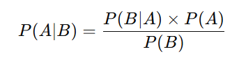
Where:
| Term | Meaning |
|---|---|
| P(A|B) | Posterior Probability |
| P(B|A) | Likelihood |
| P(A) | Prior Probability |
| P(B) | Evidence |
Understanding the Formula
Suppose:
A = Spam
B = Word "Free"
Then:
P(A)
Probability that an email is Spam.
Example:
40 out of 100 emails are spam
P(Spam) = 40/100 = 0.4
P(B|A)
Probability that a spam email contains the word "Free".
Suppose:
32 spam emails contain "Free"
P(Free∣Spam) = 32/40 = 0.8
P(A|B)
Probability that an email is spam given that it contains the word "Free".
This is what we want to calculate.
Working Example
Suppose we have:
| Email Type | Count |
|---|---|
| Spam | 40 |
| Not Spam | 60 |
Total Emails:
100
Step 1: Calculate Prior Probabilities
Spam
P(Spam)=40/100
Not Spam
P(NotSpam)=60/100
Step 2: Calculate Likelihood
Suppose:
| Word | Spam Emails |
|---|---|
| Free | 32 |
P(Free∣Spam)=32/40
Suppose:
| Word | Not Spam Emails |
|---|---|
| Free | 6 |
P(Free∣NotSpam)=6/60
Step 3: Apply Bayes Theorem
We compare probabilities for each class.
For Spam:
P(Spam∣Free)∝P(Free∣Spam)×P(Spam)
Substitute values:
0.8×0.4
For Not Spam:
P(NotSpam∣Free)∝P(Free∣NotSpam)×P(NotSpam)
0.1×0.6
Step 4: Compare Probabilities
| Class | Probability |
|---|---|
| Spam | 0.32 |
| Not Spam | 0.06 |
Since:
0.32 > 0.06
Prediction:
Spam
Another Example Using Student Data
Suppose we want to predict whether a student will pass an exam.
Training Data:
| Study Hours | Result |
|---|---|
| High | Pass |
| High | Pass |
| Medium | Pass |
| Low | Fail |
| Low | Fail |
Step 1: Prior Probability
Pass:
P(Pass)=3/5=0.6
Fail:
P(Fail)=2/5=0.4
Step 2: Likelihood
For a student with:
Study Hours = High
Likelihood:
P(High∣Pass)=2/3
P(High∣Fail)=0/2
Step 3: Calculate Posterior
Pass:
0.667×0.6
Fail:
0×0.40
Prediction:
Pass
How Naive Bayes Makes Predictions
Training Data
       ↓
Calculate Prior Probabilities
       ↓
Calculate Likelihood Probabilities
       ↓
Apply Bayes Theorem
       ↓
Compute Posterior Probabilities
       ↓
Select Highest Probability Class
Why Naive Bayes Works Well
Even though the independence assumption is often incorrect:
Feature Independence Assumption
Naive Bayes still performs surprisingly well because:
-
Probability calculations are simple
-
Less data is required
-
Fast training
-
Fast prediction
Advantages
-
Easy to understand
-
Fast training
-
Fast prediction
-
Works well with small datasets
-
Excellent for text classification
-
Handles high-dimensional data efficiently
Limitations
-
Assumes feature independence
-
Probability estimates may not be accurate
-
Can struggle with highly correlated features
Applications
Spam Detection
Spam / Not Spam
Sentiment Analysis
Positive / Negative
Document Classification
Sports
Politics
Technology
Business
Medical Diagnosis
Disease Prediction
Python Implementation
Example 1: Simple Naive Bayes Classification
from sklearn.naive_bayes import GaussianNB

# Training Data
X = [
    [1],
    [2],
    [3],
    [8],
    [9],
    [10]
]

y = [
    "Fail",
    "Fail",
    "Fail",
    "Pass",
    "Pass",
    "Pass"
]

# Create Model
model = GaussianNB()

# Train Model
model.fit(X, y)

# Predict
prediction = model.predict([[7]])

print("Prediction:", prediction[0])
Output:
Prediction: Pass
Example 2: Email Spam Classification
from sklearn.feature_extraction.text import CountVectorizer
from sklearn.naive_bayes import MultinomialNB

emails = [
    "Free prize winner",
    "Claim your free offer",
    "Meeting at 10 AM",
    "Project discussion tomorrow"
]

labels = [
    "Spam",
    "Spam",
    "Not Spam",
    "Not Spam"
]

vectorizer = CountVectorizer()

X = vectorizer.fit_transform(emails)

model = MultinomialNB()

model.fit(X, labels)

test_email = vectorizer.transform(
    ["Free offer available"]
)

prediction = model.predict(test_email)

print(prediction[0])
Output:
Spam
Important Points
-
Naive Bayes is a probabilistic classification algorithm.
-
It is based on Bayes Theorem.
-
It assumes all features are independent.
-
Prediction is based on posterior probabilities.
-
The class with the highest probability is selected.
-
It is extremely fast and memory efficient.
-
Widely used in spam filtering and text classification.
-
It works surprisingly well despite its naive assumption.
Keywords
Naive Bayes Classifier, Bayes Theorem, Probabilistic Classification, Prior Probability, Posterior Probability, Likelihood, Spam Detection, Machine Learning Classification, Bayesian Learning, Feature Independence Assumption