
Polynomial Regression
Polynomial Regression is a supervised machine learning algorithm used when the relationship between input and output variables is nonlinear.
In Simple Linear Regression:
Data follows a straight line
But in many real-world problems:
Data follows a curve
Polynomial Regression helps model such curved relationships.
Real-Life Example
Suppose we want to predict:
-
Salary based on experience
-
Plant growth based on temperature
-
Sales based on advertisement spending
Sometimes the output does not increase in a straight-line pattern.
Example Dataset
| Experience | Salary |
|---|---|
| 1 | 15 |
| 2 | 20 |
| 3 | 28 |
| 4 | 40 |
| 5 | 60 |
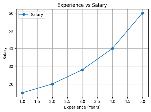
If we plot this data:
-
The relationship appears curved
-
A straight line cannot fit properly
Why Polynomial Regression is Needed
Linear Regression works well only when:
Input and output have a linear relationship
But real-world data often contains:
-
Curves
-
Nonlinear trends
-
Complex patterns
Polynomial Regression converts linear models into nonlinear models by adding powers of input variables.
Polynomial Regression Equation
Degree 2 Polynomial
y = b0 + b1x + b2x²
Degree 3 Polynomial
y = b0 + b1x + b2x² + b3x³
Where:
-
y → Predicted output
-
x → Input feature
-
b0 → Intercept
-
b1, b2, b3 → Coefficients
Understanding Polynomial Features
Suppose:
x = 2
Then:
x² = 4
x³ = 8
These additional powers help the model capture curved relationships.
Mathematical Example
Suppose the model equation is:
y = 2 + 3x + x²
Predict output for:
x = 4
Substitute values:
y = 2 + 3(4) + (4²)
Calculate:
3(4) = 12
4² = 16
Final value:
y = 2 + 12 + 16
y = 30
Visual Difference
Linear Regression
Straight Line
Polynomial Regression
Curved Line
Practical Example Using Python
Step 1: Import Libraries
import numpy as np
import pandas as pd
import matplotlib.pyplot as plt

from sklearn.linear_model import LinearRegression
from sklearn.preprocessing import PolynomialFeatures
Step 2: Create Dataset
data = {
    "Experience": [1, 2, 3, 4, 5],
    "Salary": [15, 20, 28, 40, 60]
}

df = pd.DataFrame(data)

print(df)
Step 3: Define Features and Target
X = df[["Experience"]]
y = df["Salary"]
Step 4: Convert to Polynomial Features
poly = PolynomialFeatures(degree=2)

X_poly = poly.fit_transform(X)
This creates:
x and x² features
Step 5: Train Model
model = LinearRegression()

model.fit(X_poly, y)
Step 6: Predict New Value
Predict salary for:
Experience = 6
prediction = model.predict(poly.transform([[6]]))

print(prediction)
Expected Output
[80.]
Step 7: Visualize Polynomial Curve
plt.scatter(df["Experience"], df["Salary"])

x_range = np.linspace(1, 5, 100).reshape(-1,1)

plt.plot(
    x_range,
    model.predict(poly.transform(x_range)),
    color="red"
)

plt.xlabel("Experience")
plt.ylabel("Salary")

plt.title("Polynomial Regression")

plt.show()
Understanding the Graph
-
Blue dots → Actual data points
-
Red curve → Polynomial regression curve
The curve fits nonlinear data better than a straight line.
Degree of Polynomial
| Degree | Shape |
|---|---|
| 1 | Straight line |
| 2 | Simple curve |
| 3 | More complex curve |
| Higher Degree | More flexible curve |
Important Point
Higher degree:
-
Increases flexibility
-
May cause overfitting
Choosing the correct degree is important.
Advantages
-
Handles nonlinear data
-
Better curve fitting
-
Improves prediction accuracy
-
Easy extension of Linear Regression
Limitations
-
Higher degree may overfit
-
Sensitive to outliers
-
Complex interpretation
Real-World Applications
| Application | Usage |
|---|---|
| Salary Prediction | Experience vs Salary |
| Stock Market Analysis | Trend prediction |
| Sales Forecasting | Nonlinear sales patterns |
| Biology | Growth curve analysis |
Important Interview Points
1. Polynomial Regression models nonlinear relationships.
2. Polynomial features add powers of input variables.
3. Degree controls curve complexity.
4. Higher polynomial degree may cause overfitting.
5. Polynomial Regression is built on Linear Regression.
Summary
Polynomial Regression is a supervised learning algorithm used to model nonlinear relationships between input and output variables. It extends Linear Regression by adding polynomial features, allowing the model to fit curved data patterns more effectively.