Single Layer Perceptron - Machine Learning

Before learning Multi-Layer Perceptrons and Neural Networks, it is important to understand the Single Layer Perceptron, which is the simplest neural network model.

It was introduced by Frank Rosenblatt in 1958 and is considered the foundation of modern neural networks.

What is a Single Layer Perceptron?

A Single Layer Perceptron is a supervised learning algorithm used for binary classification.

Its goal is:

Learn a linear decision boundary that separates two classes.

It is one of the earliest machine learning classification algorithms.

Biological Inspiration

The perceptron is inspired by the human brain neuron.

Biological neuron:

Inputs
   ↓
Neuron
   ↓
Output

Perceptron:

Features
   ↓
Weighted Sum
   ↓
Activation Function
   ↓
Prediction

Structure of Single Layer Perceptron

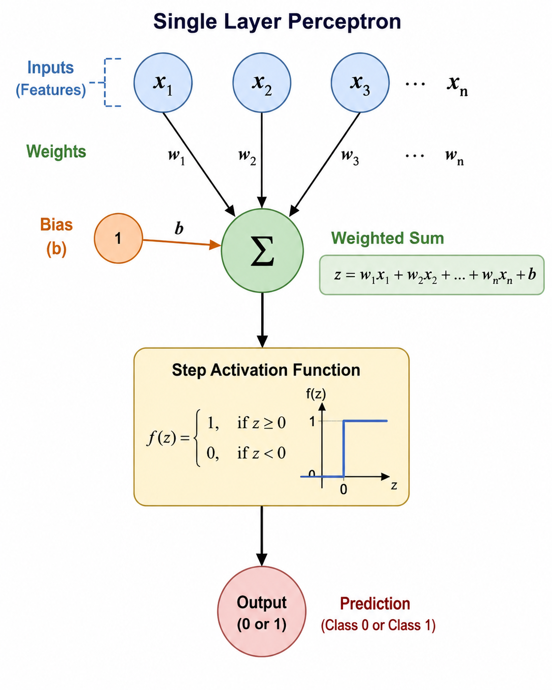
Where:

x1,x2,x3 = Inputs
w1,w2,w3 = Weights
b         = Bias

The Single Layer Perceptron processes input features through a series of steps to make a binary classification prediction. Each input feature (x₁, x₂, x₃, ..., xₙ) is multiplied by its corresponding weight (w₁, w₂, w₃, ..., wₙ), which represents the importance of that feature. A bias term (b) is also added to the weighted inputs.

The perceptron then computes the weighted sum:

z = w1x1 + w2x2 +⋯ + wnxn+b

This weighted sum is passed through a Step Activation Function, which acts as a decision-maker. If the value of zz is greater than or equal to zero, the perceptron outputs 1; otherwise, it outputs 0.

Thus, the perceptron converts multiple input features into a single binary prediction, making it suitable for simple classification tasks where data can be separated using a straight-line decision boundary.

How Perceptron Works

The perceptron performs three steps:

Step 1: Weighted Sum

Calculate:

z = w1x1 + w2x2 +⋯ + wnxn+b

This combines all input features.

Step 2: Apply Activation Function

The perceptron uses a Step Function.

If z ≥ 0 → Output = 1

If z < 0 → Output = 0

Step 3: Generate Prediction

The output becomes the predicted class.

Example:

Output = 1 → Positive Class

Output = 0 → Negative Class

Example

Suppose:

Feature	Value
x1	2
x2	3

Weights:

w1 = 1
w2 = 2

Bias:

b = -4

Calculate Weighted Sum

z=(1)(2)+(2)(3)−4

z=2+6−4

z=4

Apply Step Function

z = 4 ≥ 0

Therefore:

Output = 1

Prediction:

Class 1

Learning Process

Initially:

Weights are random

The perceptron predicts a class.

Then:

Compare Prediction
       ↓
Calculate Error
       ↓
Update Weights
       ↓
Improve Boundary

This process repeats until classification errors become minimal.

Perceptron Learning Rule

Weight update formula:

w_new=w_old+η(y−ŷ)x

Where:

η      = Learning Rate
y      = Actual Output
ŷ      = Predicted Output
x      = Input Feature

Example of Weight Update

Suppose:

Actual Output = 1
Predicted Output = 0
Learning Rate = 0.1
Input = 2
Current Weight = 0.5

Update:

 $w_{n e w} = 0.5 + 0.1 (1 - 0) (2)$  
 $w_{n e w} = 0.5 + 0.2$  $= 0.7$

The weight increases because the model made a mistake.

Decision Boundary

The perceptron creates a linear decision boundary.

Example:

Class A     |     Class B

The boundary is always:

Straight Line

Therefore:

A Single Layer Perceptron can only solve linearly separable problems.

Limitation: XOR Problem

Consider:

x1	x2	Output
0	0	0
0	1	1
1	0	1
1	1	0

This is the XOR problem.

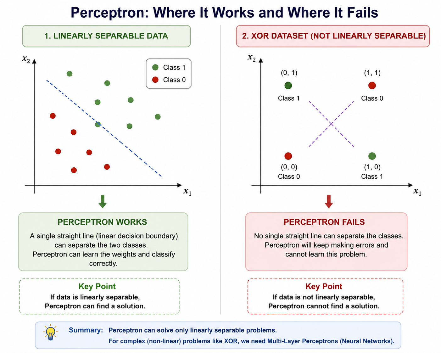
No single straight line can separate these classes.

Therefore:

Single Layer Perceptron fails

This limitation led to the development of Multi-Layer Perceptrons.

Applications

Binary classification
Pattern recognition
Character recognition
Basic neural network learning
Educational understanding of neural networks

Advantages

Simple to understand
Fast training
Easy implementation
Foundation of neural networks

Limitations

Works only for linearly separable data
Cannot solve XOR problem
Limited learning capability
Less powerful than modern neural networks

Python Implementation

from sklearn.linear_model import Perceptron

X = [[1,1],[2,2],[4,4],[5,5]]
y = [0,0,1,1]

model = Perceptron()

model.fit(X,y)

prediction = model.predict([[3,3]])

print(prediction)

Important Points

Single Layer Perceptron is the simplest neural network.
It performs binary classification.
It uses weighted inputs and a bias.
The activation function is typically a step function.
The learning rule updates weights based on prediction errors.
It creates a linear decision boundary.
It works only for linearly separable datasets.
It cannot solve the XOR problem.
It is the foundation of modern neural networks.

Keywords

Single Layer Perceptron, Perceptron Learning Rule, Artificial Neuron, Step Function, Linear Classification, Binary Classification, Weight Update, Decision Boundary, Neural Network Fundamentals, XOR Problem