Kernel Functions in SVM
In the previous tutorial, we learned that Linear SVM works well when data can be separated using a straight line (or hyperplane).
However, many real-world datasets are not linearly separable. In such situations, a straight line cannot correctly separate the classes.
To understand this problem, consider the following XOR dataset.
| x1 | x2 | Class |
|---|---|---|
| 0 | 0 | Red |
| 0 | 1 | Blue |
| 1 | 0 | Blue |
| 1 | 1 | Red |
Visual representation:
(0,1)  Blue      (1,1)  Red


(0,0)  Red       (1,0)  Blue
Notice that the classes are arranged diagonally.
No matter how we draw a straight line:
|
—
/
\
we cannot separate all Red points from all Blue points.
This means:
Linear SVM fails
because the data is not linearly separable.
Another Example: Circular Dataset
Consider the following dataset:
Outer Circle  → Red

Inner Circle  → Blue
Visual representation:
      R R R R R

    R           R

   R    B B B    R

   R    B B B    R

    R           R

      R R R R R
Here:
Blue points are surrounded by Red points.
Again, no straight line can separate all Blue points from all Red points.
Therefore:
Linear SVM cannot solve this problem.
Why Do We Need Kernels?
When data is not linearly separable, we need a way to transform it into a space where separation becomes possible.
Kernel Functions help us achieve this.
A kernel function maps the original data into a higher-dimensional space where a linear hyperplane can separate the classes.
In simple words:
A kernel transforms a non-linear problem into a linear problem in a higher-dimensional space.
Understanding the Kernel Trick
Normally, the process would be:
Original Data
      ↓
Transform to Higher Dimension
      ↓
Train Linear SVM
However, explicitly transforming every data point can be computationally expensive.
To solve this problem, SVM uses the Kernel Trick.
The Kernel Trick allows SVM to perform computations as if the data has already been transformed into a higher-dimensional space without actually performing the transformation.
Benefits:
Faster computation
Less memory usage
Efficient learning
How Kernel SVM Solves the Circular Dataset
In the original 2D space:
Outer Ring = Red
Inner Circle = Blue
The classes cannot be separated using a straight line.
After applying a kernel transformation:
Original Space (2D)
        ↓
Higher-Dimensional Space
        ↓
Linear Separation Becomes Possible
Now SVM can find a hyperplane that separates the classes.
When projected back into the original space, the decision boundary appears as a circle or curve instead of a straight line.
This is the fundamental idea behind Kernel SVM.
Major Kernel Functions in SVM
The most commonly used kernel functions are:
-
Linear Kernel
-
Polynomial Kernel
-
Radial Basis Function (RBF) Kernel
-
Sigmoid Kernel
Each kernel creates a different type of decision boundary and is suitable for different types of datasets.
Let's understand each kernel in detail.
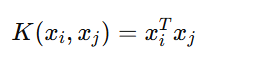
1. Linear Kernel
Idea
The Linear Kernel does not transform the data into a higher dimension.
It simply finds the best straight-line decision boundary.
Kernel Formula:
Decision Boundary
Red Class     |     Blue Class
Red Class     |     Blue Class
Red Class     |     Blue Class
The boundary is a straight line.
When to Use
-
Data is linearly separable
-
High-dimensional datasets
-
Text classification
-
Spam detection
-
Sentiment analysis
Advantages
-
Fast training
-
Simple implementation
-
Less computational cost
Limitations
-
Cannot capture non-linear relationships
2. Polynomial Kernel
Idea
The Polynomial Kernel allows SVM to learn curved decision boundaries.
Instead of using only original features, it creates combinations of features.
Kernel Formula:
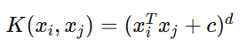
Where:
c = Constant
d = Degree of Polynomial
Example
Suppose:
x = (x1, x2)
Polynomial expansion may generate:
x1²
x2²
x1x2
These additional features help separate complex patterns.
Decision Boundary
)))))))))))))))
Curved boundaries are possible.
When to Use
-
Moderately non-linear data
-
Feature interaction problems
-
Curved patterns
Advantages
-
Captures non-linear relationships
-
More flexible than Linear Kernel
Limitations
-
Computationally expensive
-
High-degree polynomials may overfit
3. Radial Basis Function (RBF) Kernel
Idea
RBF is the most widely used kernel in practical applications.
It creates highly flexible decision boundaries and can handle very complex datasets.
Kernel Formula:
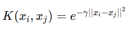
Where:
γ (Gamma) controls how far the influence of a training point extends.
How It Works
RBF measures similarity between points.
If two points are very close:
High Similarity
If two points are far apart:
Low Similarity
Decision Boundary
RBF can create:
Circles
Curves
Complex Shapes
Example:
Outer Circle  → Red

Inner Circle  → Blue
RBF can successfully separate these classes.
When to Use
-
Non-linear datasets
-
Unknown data patterns
-
Most real-world classification problems
Advantages
-
Excellent performance
-
Highly flexible
-
Works well in many practical situations
Limitations
-
Requires tuning of Gamma and C
-
Slower than Linear Kernel
4. Sigmoid Kernel
Idea
The Sigmoid Kernel behaves similarly to activation functions used in neural networks.
Kernel Formula:
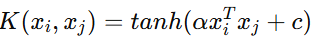
Where:
α = Scaling Parameter
c = Constant
Decision Boundary
Produces non-linear boundaries similar to neural networks.
When to Use
-
Experimental applications
-
Specialized problems
Advantages
-
Neural-network-like behavior
Limitations
-
Less commonly used
-
Often performs worse than RBF
Comparison of Kernel Functions
| Kernel | Boundary Type | Complexity | Common Usage |
|---|---|---|---|
| Linear | Straight Line | Low | Text Classification |
| Polynomial | Curved | Medium | Feature Interaction Problems |
| RBF | Highly Flexible | High | Most Real-World Problems |
| Sigmoid | Neural Network Style | Medium | Specialized Tasks |
How to Choose the Right Kernel
Use Linear Kernel When
Data is linearly separable
Large datasets
Text classification
Use Polynomial Kernel When
Moderate non-linearity exists
Feature interactions are important
Use RBF Kernel When
Data is non-linear
Pattern is unknown
Need maximum flexibility
This is usually the first choice for non-linear SVM.
Use Sigmoid Kernel When
Experimenting with neural-network-like decision boundaries
Important Points
-
Kernel functions help SVM solve non-linear problems.
-
Kernels transform data into higher-dimensional spaces.
-
The Kernel Trick avoids explicit transformation.
-
Linear Kernel creates straight decision boundaries.
-
Polynomial Kernel creates curved boundaries.
-
RBF Kernel creates highly flexible boundaries.
-
Sigmoid Kernel behaves similarly to neural networks.
-
RBF is the most commonly used kernel in practice.
-
Choosing the correct kernel greatly affects model performance.
Keywords
SVM Kernel Functions, Linear Kernel, Polynomial Kernel, RBF Kernel, Sigmoid Kernel, Kernel Trick, Non Linear SVM, Support Vector Machine Kernels, Machine Learning Classification, Decision Boundaries in SVM